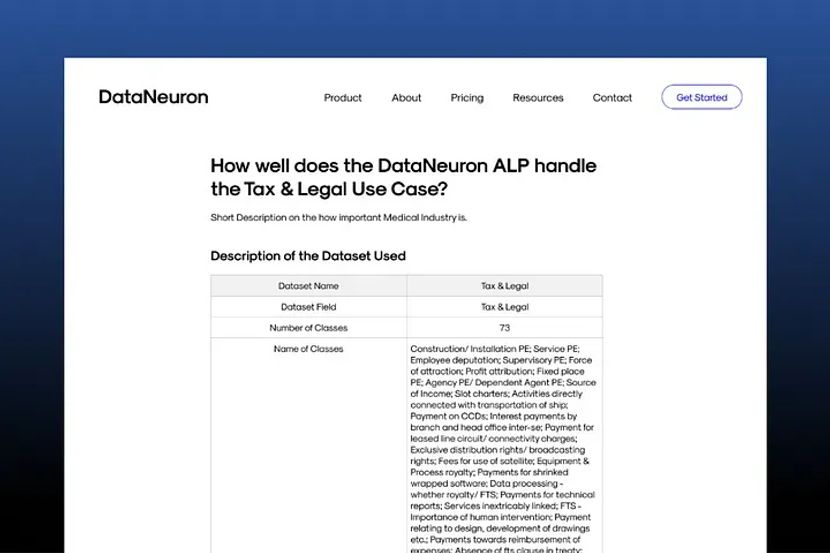
This is the table that explains the dataset that was used to conduct this case study.
Explaining the DataNeuron Pipeline
This is the DataNeuron Pipeline. Ingest, Structure, Validate, Train, Predict, Deploy and Iterate.
Results of our Experiment
Results of our Experiment
Reduction in SME Labelling Effort
During an in-house project, the SMEs have to go through all the paragraphs present in the dataset in order to figure out which paragraphs actually belong to the 73 classes mentioned above. This would usually take a tremendous amount of time and effort.
When using DataNeuron ALP, the algorithm was able to perform strategic annotation on 15000 raw paragraphs and filter out the paragraphs that belonged to the 73 classes and provide 4303 paragraphs to the user for validation. Taking as little as 45 seconds to annotate each paragraph, an in-house project would take an estimate of 187.5 hours just to annotate all the paragraphs while by using DataNeuron, it only took 35.85 hours.
Difference in paragraphs annotated between an in-house solution and DataNeuron.
Advantage of Suggestion-Based Annotation
Instead of making users go through the entire dataset to label paragraphs that belong to a certain class, DataNeuron uses a validation-based approach to make the model training process considerably easier. The platform provides the users with a list of annotated/ labelled paragraphs that are most likely to belong to the same class by using context-based filtering and analysing the masterlist. The users simply have to validate whether the system labelled paragraph belongs to the class mentioned. This validation-based approach also reduces the time it takes to annotate each paragraph. Based on our estimate, it takes approximately 30 seconds for a user to identify whether a paragraph belongs to a particular class. Based on this, it would take an estimate of 35.85 hours for the users to validate 4303 paragraphs provided by the DataNeuron ALP. When compared to the 187.5 hours it would take for an in-house team to complete the annotation process, DataNeuron offers a staggering 81% reduction in time spent.
Difference in time spent annotating between an in-house solution and DataNeuron.
The Accuracy Achieved
When conducting this case study, the accuracy we achieved for the model trained by the DataNeuron ALP was 87% which, considering the high number of classes and small number of training paragraphs, proves to work very well in real world scenarios. The accuracy of the model trained by the DataNeuron ALP can be improved by validating more paragraphs or by adding seed paragraphs.
Calculating the Cost ROI
The number of paragraphs that needs to be annotated in an in-house project is 15000 and it would cost approximately $3280. The number of paragraphs that needs to be annotated when using the DataNeuron ALP is 4303 since most of the paragraphs which did not belong to any of 73 classes were discarded using context-based filtering. The cost for annotating 4303 paragraphs using the DataNeuron ALP is $976.85.
Difference in cost between an in-house solution and DataNeuron.
No Requirement for a Data Science/Machine Learning Expert
The DataNeuron ALP is designed in such a way that no prerequisite knowledge of data science or machine learning is required to utilize the platform to its maximum potential.
For some very specific use cases, a Subject Matter Expert might be required but for the majority of use cases, an SME is not required in the DataNeuron Pipeline.
DataNeuron is thrilled to announce the official launch of the DataNeuron Automated Learning Platform (ALP). The ALP has been strategically designed to accelerate and automate human-in-loop annotation for developing AI solutions. Powered by a data-centric platform, we automate data labeling, the creation of models, and end-to-end lifecycle management of ML.
We are a team of Data Science enthusiasts having first-hand experience of dealing with data analysts, subject matter experts and data scientists to fulfil the labelled data requirements for building highly accurate contextual algorithms for various use-cases. Our aim is to accelerate the development and provide better explainability of AI.
We are also excited to partner with leading venture capitalists, angel investors and strategic advisors in expanding the horizons of DataNeuron.
But why should we switch from human labelling to the DataNeuron ALP? That’s a great question! Based on our findings from the case studies we have conducted, we have found out that using the DataNeuron ALP can reduce the time spent in annotating by a staggering 89.10%, reduce the number of paragraphs validated by 83.55%, reduce the cost expenditure by 77.83% and yield an ROI of an astounding 372.22%.
The DataNeuron Pipeline
Those numbers sound promising but what more can we do on the DataNeuron ALP? Once Again, that’s a great question! Apart from getting accurately labelled data, the DataNeuron ALP can be used to perform no-code prediction. With just a click of a button, the platform can be used to make a prediction on any new paragraphs in exchange for a very minimal fee. This does not require any knowledge of programming and users can utilize this service for any input data from the platform. This can also be integrated into other platforms by making use of the exposed prediction API or the deployed Python package.
As a cherry on top, the DataNeuron ALP is designed in such a way that no prerequisite knowledge of data science or machine learning is required to utilize the platform to its maximum potential. The users only need some knowledge of the domain they are working on and the details of the project and they’re good to go! For some very specific use cases, a Subject Matter Expert might be required but for the majority of use cases, an SME is not required in the DataNeuron Pipeline.
The sample is a collection of people, things, or things used in the study that is taken for analysis from a wider population. To enable us to extrapolate the research sample’s findings to the entire population, the sample must be representative of the population.
Let’s go through a real-world scenario.
We’re looking for Mumbai’s adult population’s average annual salary. Up till 2022, Mumbai has a population of about 30 million. Males and females in this population would roughly be split 1:1 (these are simple generalizations), and they might have different averages. Similarly, there are numerous more ways in which various adult population groupings may have varying income levels. As you may guess, it is incredibly difficult to determine the average adult income in Mumbai.
Since it’s impossible to reach every adult in the whole population, what can be the solution? We can collect numerous samples and determine the average height of the people in the chosen samples.
How can we take a Sample?
Taking the same scenario from above, imagine we only take samples from the people in managerial positions. This won’t be regarded as a decent sample because, on generalizing, a manager earns more than the average adult, and it will provide us with a poor estimation of the income of the average adult. A sample must accurately reflect the universe from which it was drawn.
There are various different potential solutions, but we’ll be looking at three major techniques.
Sampling strategies :
Most uncertain probability
Most certain data points
The basic mixture from different confidence intervals
Most Uncertain Probability
The aim behind uncertainty sampling is to focus on the data item that the present predictor is least certain about. To put it another way, uncertainty sampling typically finds points that are located near thWhat is Sampling?
The sample is a collection of people, things, or things used in the study that is taken for analysis from a wider population. To enable us to extrapolate the research sample’s findings to the entire population, the sample must be representative of the population.
Let’s go through a real-world scenario.
We’re looking for Mumbai’s adult population’s average annual salary. Up till 2022, Mumbai has a population of about 30 million. Males and females in this population would roughly be split 1:1 (these are simple generalizations), and they might have different averages. Similarly, there are numerous more ways in which various adult population groupings may have varying income levels. As you may guess, it is incredibly difficult to determine the average adult income in Mumbai.
Since it’s impossible to reach every adult in the whole population, what can be the solution? We can collect numerous samples and determine the average height of the people in the chosen samples.
How can we take a Sample?
Taking the same scenario from above, imagine we only take samples from the people in managerial positions. This won’t be regarded as a decent sample because, on generalizing, a manager earns more than the average adult, and it will provide us with a poor estimation of the income of the average adult. A sample must accurately reflect the universe from which it was drawn.
There are various different potential solutions, but we’ll be looking at three major techniques.
Sampling strategies :
Most uncertain probability
Most certain data points
The basic mixture from different confidence intervals
Most Uncertain Probability
The aim behind uncertainty sampling is to focus on the data item that the present predictor is least certain about. To put it another way, uncertainty sampling typically finds points that are located near the decision boundary of the current model.
Uncertainty Sampling
Assume that a student is preparing for an exam and has 1000 questions to go through. The student only has time to go through 100 of them. Naturally, the student should prepare 100 questions on which the individual is least confident. With the new questions, students should get smarter, and faster.
Most Certain Data Points
This method chooses the data points with the highest certainty ie. data points that are predicted by the model with the highest confidence. These data points have maximum chances of getting correctly predicted by the model. Such data points may or may not add a lot of new information to the model learning.
Basic mixture of different Confidence Intervals
Data points are grouped according to their confidence scores, and sampling is done from all of these intervals or groups. This way, we can make sure that no kind of data is missed out upon. This ensures that the sampled data points are having a balance of certain and uncertain data points. This way the model can learn the decision boundary well without missing out on already learned information.
Code
Now, let’s use these sampling methods and see their application using a simple code in Python!
We’ll be working with a binary classification problem, using two datasets:
IMDB Movie Review Dataset for sentiment analysis. Two classes in this dataset: Positive, Negative
Emotion Dataset. Two classes in this dataset: Joy, Sadness
We have performed this experiment on Jupyter Notebook.
Loading Data & Preprocessing
The availability of data is always a determining factor in the field of machine learning, so loading data should be done first. After loading the dataset and the necessary modules, the dataframe should be looking like this.
Clean the data by replacing all occurrences of breaks with single white space.
for idx in range(len(df['review'])):
    df['review'][idx] = df['review'][idx].replace('<br /><br />', ' ')
For ease of the experiment, we’re using 10k paragraphs out of the whole dataset of 50k paragraphs.
Since the train and test sets have been constructed, the pipeline can be instantiated. The pipeline consists of three steps: data transformation, resampling, and model creation at the end.
# The resulting matrices will have the shape of (`nr of examples`, `nr of word n-grams`)
vectorizer = CountVectorizer(ngram_range=(1, 5))
X_100_train = vectorizer.fit_transform(df_100_train.review)
X_stage1_test = vectorizer.transform(df_stage1_test.review)
X_test = vectorizer.transform(df_test.review)

labelencoder = LabelEncoder()
df_100_train['sentiment'] = labelencoder.fit_transform(df_100_train['sentiment'])
df_stage1_test['sentiment'] = labelencoder.transform(df_stage1_test['sentiment'])
df_test['sentiment'] = labelencoder.transform(df_test['sentiment'])
Before moving on to sampling strategies, an initial model is trained
1000 or more paragraphs are picked from a window of probability with the highest degree of uncertainty. These 1000 paragraphs are sorted increasingly in a dataframe. Then we compute the predicted probability’s mean value.
The index of the row with the predicted probability value closest to the mean value is calculated.
The paragraph sets are chosen using the mean value index row (Half of them from greater than part and half of them from less than part of the probability). To choose the most uncertain sets of paragraphs, use the same method as minimizing and maximizing the uncertain probability window range.
#index of the row closest to the mean value of predicted probability

mid_idx = int(len(df_uncertain_sorted)/2)
mean_idx = mid_idx-12
df_uncertain_sorted['predict_proba'].mean()
[Out]: 0.4936057560087512
num_of_para = [100,200,300,400,500,600,700,800,900,1000]
score_uncertain_list = []

for para in num_of_para:

    para_idx = int(para/2)

    #training set
    df_uncertain_new = df_uncertain_sorted.iloc[mean_idx-para_idx:mean_idx+para_idx]

    #preprocessing
    X_train_uncertain = vectorizer.transform(df_uncertain_new.review)

    #defining the classifier
    logreg_uncertain = LogisticRegression()

    #training the classifier
    logreg_uncertain.fit(X=X_train_uncertain, y=df_uncertain_new['sentiment'].to_list())
    #calculating the accuracy score on the test set
    score_uncertain = logreg_uncertain.score(X_test, df_test['sentiment'].to_list())
    score_uncertain_list.append(score_uncertain)

score_uncertain_list
[Out]: [0.547, 0.5845, 0.584, 0.612, 0.6215, 0.6335, 0.6415, 0.663, 0.659, 0.6755]
Most Certain Probability Sampling
The dataframe with 7900 paragraphs is sorted in descending order of their predicted probabilities. The top [100,200,300,400,500,600,700,800,900,1000] sets of paragraphs are selected as the most certain paragraphs.
num_of_para = [100,200,300,400,500,600,700,800,900,1000]
score_certain_list = []

for para in num_of_para:

    #training set
    df_certain = df_proba_sorted[:para]

    #preprocessing
    X_train_certain = vectorizer.transform(df_certain.review)

    #defining the classifier
    logreg_certain = LogisticRegression()

    #training the classifier
    logreg_certain.fit(X=X_train_certain, y=df_certain['sentiment'].to_list())

    #calculating the accuracy score on the test set
    score_certain = logreg_certain.score(X_test, df_test['sentiment'].to_list())

    score_certain_list.append(score_certain)

score_certain_list
[Out]: [0.5215, 0.54, 0.536, 0.5755, 0.5905, 0.6245, 0.641, 0.6735, 0.7355, 0.7145]
Confidence Interval Grouping Sampling
In this method, the 25th and 75th percentile of the predicted probabilities are calculated. Then the 7900 paragraphs are separated into 3 groups.
From these 3 groups [100,200,300,400,500.600,700.800.900,1000] sets of paragraphs are sampled out according to these fractions:
#calculating the 25th and 75th percentile

proba_arr = df_proba['predict_proba']
percentile_75 = np.percentile(proba_arr, 75)
percentile_25 = np.percentile(proba_arr, 25)

print("25th percentile of arr : ",
       np.percentile(proba_arr, 25))
[Out]: 25th percentile of arr :  0.28084100127515504
print("75th percentile of arr : ",
       np.percentile(proba_arr, 75))
[Out]: 75th percentile of arr :  0.7063559972435552

#grouping of the paragraphs for following window
# group 1 : >= 75
df_group_1 = df_proba[df_proba['predict_proba'] >= percentile_75]
# group 2 : <75 and >= 25
df_group_2 = df_proba[(df_proba['predict_proba'] >= percentile_25) & (df_proba['predict_proba'] < percentile_75)]
# group 3 : < 25
df_group_3 = df_proba[(df_proba['predict_proba'] < percentile_25)]

df_group_1.shape, df_group_2.shape, df_group_3.shape
[Out]: ((1975, 3), (3950, 3), (1975, 3))
Four different models are then trained on each set of paragraphs for each of the 3 sampling techniques. [total 10 x 3 = 30 models]. The accuracy score is calculated for each of the cases by fitting the models on the 2000-paragraph test set.
num_of_para = [100,200,300,400,500,600,700,800,900,1000]
score_conf_list = []

#fractions
frac1 = 0.4
frac2 = 0.3
frac3 = 0.3

#sampling paragraphs from the 3 groups
df_group_1_frac = df_group_1.sample(frac=frac1, random_state=1).reset_index(drop = True)
df_group_2_frac = df_group_2.sample(frac=frac2, random_state=1).reset_index(drop = True)
df_group_3_frac = df_group_3.sample(frac=frac3, random_state=1).reset_index(drop = True)

for para in num_of_para:

    #sampling paragraphs from the 3 groups to build the training set
    df_group_1_new = df_group_1_frac[:int(frac1 * para)]
    df_group_2_new = df_group_2_frac[:int(frac2 * para)]
    df_group_3_new = df_group_3_frac[:int(frac3 * para)]

    df_list = [df_group_1_new, df_group_2_new, df_group_3_new]

    #training set
    df_conf = pd.concat(df_list).reset_index(drop = True)

    #preprocessing
    X_train_conf = vectorizer.transform(df_conf.review)

    #defining the classifier
    logreg_conf = LogisticRegression()

    #training the classifier
    logreg_conf.fit(X=X_train_conf, y=df_conf['sentiment'].to_list())

    #calculating the accuracy score on the test set
    score_conf = logreg_conf.score(X_test, df_test['sentiment'].to_list())
    score_conf_list.append(score_conf)

score_conf_list
[Out]: [0.6525, 0.6835, 0.7235, 0.7525, 0.766, 0.7735, 0.778, 0.7875, 0.796, 0.807]
Results and Conclusion
The accuracies of the three sampling strategies can now be compared, and it is clear that a combination of different confidence intervals performs better than the others. This shows that along with learning new information from uncertain paragraphs the model also requires retaining the previously learned information. Therefore a balance of data from different confidence intervals helps the model learn, maximizing the resulting overall accuracy.
This is the table that explains the dataset that was used to conduct this case study.
Explaining the DataNeuron Pipeline
This is the DataNeuron Pipeline. Ingest, Structure, Validate, Train, Predict, Deploy and Iterate.
Results of our Experiment
Results of our Experiment
Reduction in SME Labeling Effort
During an in-house project, the SMEs have to go through all the paragraphs present in the dataset in order to figure out which paragraphs actually belong to the 23 classes mentioned above. This would usually take a tremendous amount of time and effort.
When using DataNeuron ALP, the algorithm was able to perform strategic annotation on 13810 raw paragraphs and filter out the paragraphs that belonged to the 23 classes and provide 2069 paragraphs to the user for validation.
Taking as little as 45 seconds to annotate each paragraph, an in-house project would take an estimate of 173 hours just to annotate all the paragraphs.
Difference in paragraphs annotated between an in-house solution and DataNeuron.
Advantage of Suggestion-Based Annotation
Instead of making users go through the entire dataset to label paragraphs that belong to a certain class, DataNeuron uses a validation-based approach to make the model training process considerably easier.
The platform provides the users with a list of annotated/ labeled paragraphs that are most likely to belong to the same class by using context-based filtering and analysing the masterlist. The users simply have to validate whether the system labeled paragraph belongs to the class mentioned.
This validation-based approach also reduces the time it takes to annotate each paragraph. Based on our estimate, it takes approximately 30 seconds for a user to identify whether a paragraph belongs to a particular class.
Based on this, it would take an estimate of 17.25 hours for the users to validate 2069 paragraphs provided by the DataNeuron ALP. When compared to the 173 hours it would take for an in-house team to complete the annotation process, DataNeuron offers a staggering 90% reduction in time spent.
Difference in time spent annotating between an in-house solution and DataNeuron.
The Accuracy Tradeoff
When conducting this case study, the accuracy we achieved for the model trained by the DataNeuron ALP was 93.9% while the accuracy of model trained by the in-house project was 98.2%.
The accuracy of the model trained by the DataNeuron ALP can be increased by validating more paragraphs.
Difference in accuracy between an in-house solution and DataNeuron.
Calculating the Cost ROI
The number of paragraphs that needs to be annotated in an in-house project is 15067 and it would cost approximately $3288.
The number of paragraphs that needs to be annotated when using the DataNeuron ALP is 659 since most of the paragraphs which did not belong to any of 8 classes were discarded using context-based filtering. The cost for annotating 659 paragraphs using the DataNeuron ALP is $575.
The reduction in cost is a significant 82.5% and the cost ROI is an estimated 471.82%.
Difference in cost between an in-house solution and DataNeuron.
No Requirement for a Data Science/Machine Learning Expert.
The DataNeuron ALP is designed in such a way that no prerequisite knowledge of data science or machine learning is required to utilize the platform to its maximum potential.
For some very specific use cases, a Subject Matter Expert might be required but for the majority of use cases, an SME is not required in the DataNeuron Pipeline.
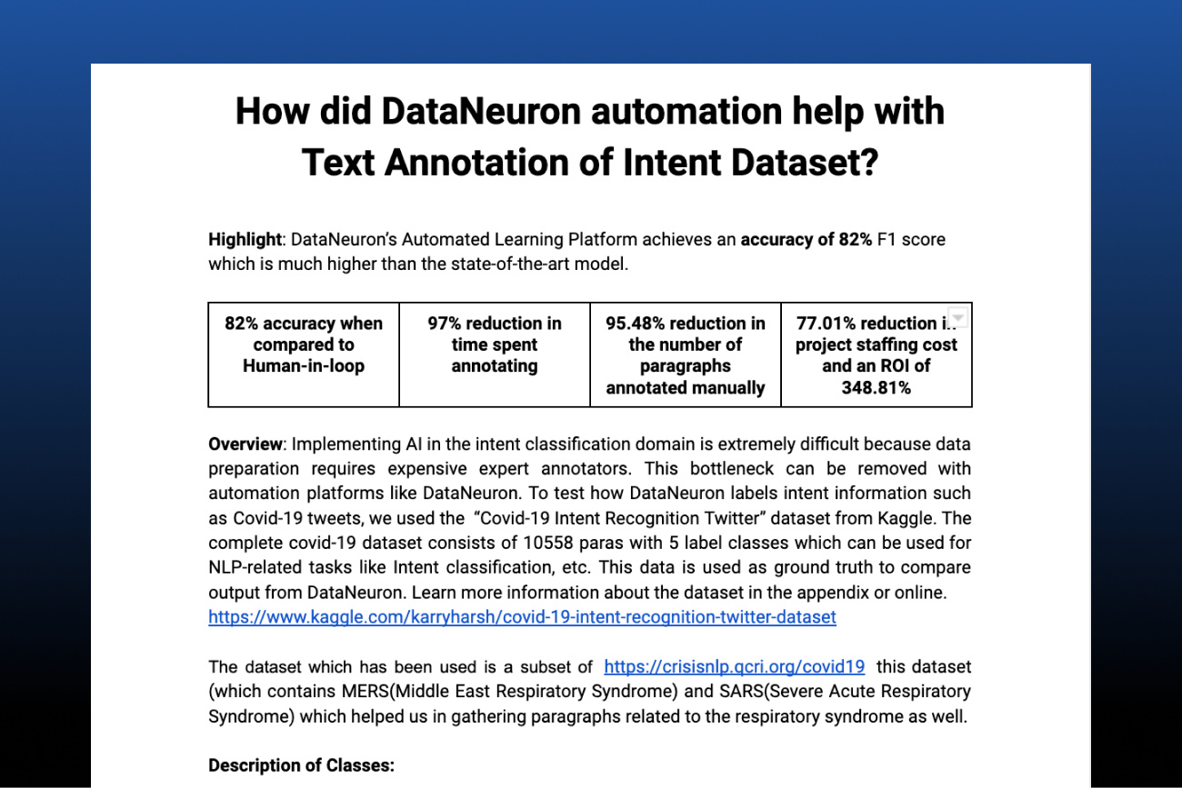
Highlight: DataNeuron’s Automated Learning Platform achieves an accuracy of 82% F1 score which is comparable to the best performing model.
Overview: Because data preparation necessitates the use of expensive expert annotators, implementing AI in the intent classification domain is exceedingly difficult. Automation platforms like DataNeuron can help eliminate this barrier. We used Kaggle’s “Covid-19 Intent Recognition Twitter” dataset to see how DataNeuron identifies intent information like Covid-19 tweets. The entire Covid-19 dataset has 10558 paras divided into 5 classes that can be utilized for NLP tasks such as intent categorization. This data serves as a baseline against which DataNeuron’s output can be compared. More information on the dataset can be found in the appendix or on the internet.
A subset of https://crisisnlp.qcri.org/covid19 was used in this study. This dataset (which includes MERS (Middle East Respiratory Syndrome) and SARS (Severe Acute Respiratory Syndrome)) assisted us in compiling paragraphs on respiratory syndromes.
Class Description:
The masterlist is made up of classes and their associated keywords, which are intuitively written against their classes and serve as inputs for our platform. We train our model on the following classes: disease_signs_or_symptoms, disease_transmission, deaths_reports, prevention, and treatment.
Background on the DataNeuron Automated Learning Platform:
The Automated Learning Platform (ALP) from DataNeuron is designed to ingest unstructured data like these Covid-19 tweets, build AI models with minimal human validation, and predict labels with high accuracy. The diagram below depicts DataNeuron’s ALP Flow
The platform performs automatic annotation and provides the users with a list of annotated paragraphs. The users simply have to validate whether the annotation is correct or incorrect. Instead of making users go through the entire dataset to label paragraphs, DataNeuron offers this validation-based approach which reduces the time taken to annotate each paragraph. Based on our estimate, it takes approximately 30 seconds for a user to identify whether a paragraph belongs to a particular class.
The Covid-19 data was fed into DataNeuron’s ALP flow, where a combination of machine learning models was built based on the input. In the first stage, these models were able to identify irrelevant paragraphs out of the 10558 raw paragraphs. The remaining relevant paragraphs were strategically annotated with one of the 5 target classes. User validation was required on 477 annotated paragraphs to achieve remarkable accuracy.
Simplifying SME Task:
With this same data, SMEs for human-in-loop labeling would have to go through each paragraph in the entire dataset to label with a target class. This exercise would take a tremendous amount of time and effort. DataNeuron’s recognize vs recall approach simplifies the validator’s task to a large extent.
Manual Effort Reduction:
Conservatively assuming 45 seconds are needed to manually annotate each paragraph, it would take 132 hours to manually annotate the complete dataset. Assuming it takes 30 seconds to validate one paragraph on DataNeuron, 477 paragraphs will take 4 hours for complete validation. This calculates to a 97% reduction in human effort required.
Accuracy close to the best classifier model:
In another experiment, the SVM model was used to classify the paragraphs in this dataset. An overall 86.0% Precision at 85% Recall (85% F-1 score) was achieved. With 477 paragraphs for manual validation, which is just 4.51% of the raw data, DataNeuron was able to achieve a comparable F-1 score of 82%.
Calculating the Cost ROI:
The Annotation cost for the in-house data team is $1320 and for the Data-Science team, it is around $1405. Therefore, the total cost is $2725. The cost for annotating 477 paragraphs using the DataNeuron ALP is around $607.3. In this case, the reduction in cost is 77.71%, which is very significant with a cost ROI of 348.81%.
No requirement for a Data Science/Machine Learning Expert:
The DataNeuron ALP by design eliminates prerequisite knowledge of data science or machine learning to utilize the platform to its maximum potential. The only human intervention is to validate the output of the labeled data.
Conclusion:
From the above explanation, it is evident that automating data labeling using DataNeuron provides comparable accuracy with reduced human efforts and cost.
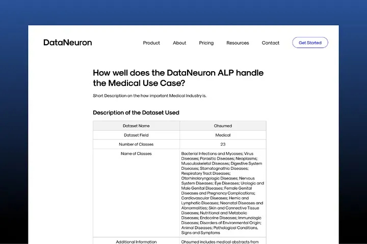
This is the table that explains the dataset that was used to conduct this case study.
Explaining the DataNeuron Pipeline
This is the DataNeuron Pipeline. Ingest, Structure, Validate, Train, Predict, Deploy and Iterate.
Results of our Experiment
Results of our Experiment
Reduction in SME Labeling Effort
During an in-house project, the SMEs have to go through all the paragraphs present in the dataset in order to figure out which paragraphs actually belong to the 8 classes mentioned above. This would usually take a tremendous amount of time and effort.
When using DataNeuron ALP, the algorithm was able to perform strategic annotation on 15000 raw paragraphs and filter out the paragraphs that belonged to the 8 classes and provide 659 paragraphs to the user for validation.
Taking as little as 45 seconds to annotate each paragraph, an in-house project would take an estimate of 188 hours just to annotate all the paragraphs.
Difference in paragraphs annotated between an in-house solution and DataNeuron.
Advantage of Suggestion-Based Annotation
Instead of making users go through the entire dataset to label paragraphs that belong to a certain class, DataNeuron uses a validation-based approach to make the model training process considerably easier.
The platform provides the users with a list of annotated/labeled paragraphs that are most likely to belong to the same class by using context-based filtering and analyzing the masterlist. The users simply have to validate whether the system labeled paragraph belongs to the class mentioned.
This validation-based approach also reduces the time it takes to annotate each paragraph. Based on our estimate, it takes approximate 30 seconds for a user to identify whether a paragraph belongs to a particular class.
Based on this, it would take an estimate of 6 hours for the users to validate 659 paragraphs provided by the DataNeuron ALP. When compared to the 188 hours it would take for an in-house team to complete the annotation process, DataNeuron offers a staggering 96.8% reduction in time spent.
Difference in time spent annotating between an in-house solution and DataNeuron.
The Accuracy Tradeoff
When conducting this case study, the accuracy we achieved for the model trained by the DataNeuron ALP was 93.9% while the accuracy of model trained by the in-house project was 98.2%.
The difference in time spent annotating could offset this small difference in accuracy and the accuracy of the model trained by the DataNeuron ALP can be increased by validating more paragraphs.
Difference in accuracy between an in-house solution and DataNeuron.
Calculating the Cost ROI
The number of paragraphs that needs to be annotated in an in-house project is 15067 and it would cost approximately $3288.
The number of paragraphs that needs to be annotated when using the DataNeuron ALP is 659 since most of the paragraphs which did not belong to any of 8 classes were discarded using context-based filtering. The cost for annotating 659 paragraphs using the DataNeuron ALP is $575.
The reduction in cost is a significant 82.5% and the cost ROI is an estimated 471.82%.
Difference in cost between an in-house solution and DataNeuron.
No Requirement for a Data Science/Machine Learning Expert
The DataNeuron ALP is designed in such a way that no prerequisite knowledge of data science or machine learning is required to utilize the platform to its maximum potential.
For some very specific use cases, a Subject Matter Expert might be required but for the majority of use cases, an SME is not required in the DataNeuron Pipeline.