Natural language querying changes everything about how businesses interact with their data. Ask a question in plain English. Get a precise, human-readable answer from your enterprise database in seconds. No SQL expertise. No analyst in the loop. No waiting days for a report. That is what DataNeuron does — and it is exactly what modern enterprises need.
But as we pushed this capability deeper into enterprise environments — HR systems, finance departments, operations teams — a hard question kept surfacing.
The query is secure. The database is secure. But what about the answer?
When DataNeuron responds to “Who are the highest-paid employees in our Chicago office?” with a clean, readable NLP paragraph, that answer has to travel somewhere. It crosses a network. It lands in a browser. It renders on a screen. And from the moment it is decrypted at the application layer, it is plain text — readable by anyone who can see that screen, intercept that session, or access that browser tab.
TLS handles data in transit. AES handles data at rest. Neither protects data at the point of display. This is the last-mile exposure problem — one of the most underappreciated attack surfaces in enterprise AI today.
We decided to solve it.
THE PROBLEM IN REAL TERMS
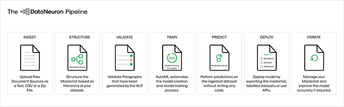
What DataNeuron actually surfaces — and why it matters
To understand the stakes, consider what DataNeuron surfaces in a typical enterprise session. In our proof of concept, we connected DataNeuron to a 50,000-record employee dataset — names, departments, locations, salaries, performance scores, shift assignments, and joining dates. The kind of data that sits behind most enterprise HR and operations systems.
A single natural language query like “Which employees have the highest performance scores?” returns a precise, readable paragraph containing names, scores, and professional details. That paragraph, once rendered in the browser, is exposed to every layer above the encryption stack — the OS, browser extensions, screen recording tools, shoulder surfing, and any hijacked or unattended session.
The compliance implications are immediate. GDPR, HIPAA, SOC 2, and the emerging AI governance frameworks Gartner has been documenting all require that sensitive data be accessible only to authorized personnel. A readable NLP answer on an unattended screen is a violation waiting to happen.
SecureFonts solves the part that everyone else ignores.
THE TECHNICAL INTEGRATION
How SecureFonts sits between DataNeuron and the browser
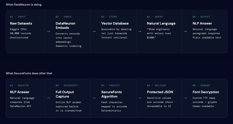
The two-pipeline architecture is what makes this work. DataNeuron handles the query and retrieval. SecureFonts intercepts the output before it is transmitted.
The SecureFonts algorithm
SecureFonts applies a deterministic, key-based unicode remapping (MUGS: Multi-Unicode Glyph Substitution) to the NLP answer at the server layer — before transmission. The substitution is:
- Deterministic — the same input with the same key always produces the same output.
- Reversible — the authorized font file maps the substituted glyphs back to readable text at render time.
- Non-reversible without the key — without the correct font, the substituted characters render as unrecognizable glyphs.
The integration flow
Connecting DataNeuron to SecureFonts required solving one specific challenge: DataNeuron’s API is asynchronous. Queries do not return immediately. The flow works as follows:
- The integration server forwards the natural language query to DataNeuron’s endpoint and receives a task ID immediately.Query Submission —
- The server polls DataNeuron’s status endpoint every three seconds until SUCCESS is returned, along with the full NLP answer and the SQL query that generated it.Async Polling —
- The NLP answer is passed through the MUGS bridge server-side. Every character is remapped before the response leaves the server.SecureFonts Protection —
- Both the raw answer and the protected version are returned to the frontend in a single JSON response. The SQL query is included in plain text for audit purposes.Dual Output —
- Authorized users with the font key loaded read the protected version as normal text. Everyone else sees unicode.Rendering —
THE THREE GARTNER USE CASES
What this pilot actually validates
Gartner’s “Implement AI Security in the Generative AI Workflow” (October 2025) identifies six stages where AI pipelines create data exposure risk. This pilot directly addresses three of them — each demonstrated live on the page with a real DataNeuron query against the real employee dataset.
USE CASE 01 · SAFE AI INGESTION
“Ensure data ingested by the AI workflow is safe through foundational controls.” — Gartner
When DataNeuron queries the employee dataset, it returns a natural language answer containing sensitive information in plain text. Without SecureFonts, that answer enters the AI pipeline as readable data — the model learns it, it gets logged, it gets cached. Every AI model trained on this data permanently absorbs whatever it ingests. Once in, there is no taking it out.
With SecureFonts active, the answer is protected before it ever leaves the integration server. The AI pipeline receives and processes unicode — it runs normally, the query works — but the sensitive values never enter the pipeline as readable text.
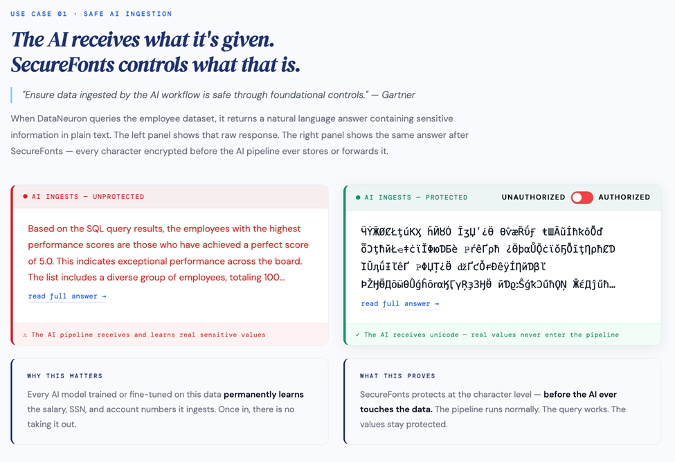
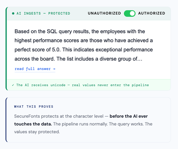
The authorized user toggles the right panel to “Authorized” and reads the answer normally through the font key. The unauthorized view — what any scraper, interceptor, or AI model without the key receives — is pure unicode.
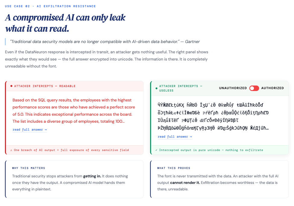
USE CASE 02 · AI EXFILTRATION RESISTANCE
“Traditional data security models are no longer compatible with AI-driven data behavior.” — Gartner
Even if the DataNeuron response is intercepted in transit — a compromised session, a man-in-the-middle, a rogue browser extension — the attacker gets nothing useful. The right panel shows exactly what they would see: the full answer encrypted into unicode.
Traditional security stops attackers from getting in. It does nothing once they have the output. A compromised AI model hands them everything in plaintext. SecureFonts means exfiltration becomes worthless — the data is there, the attacker cannot render it.
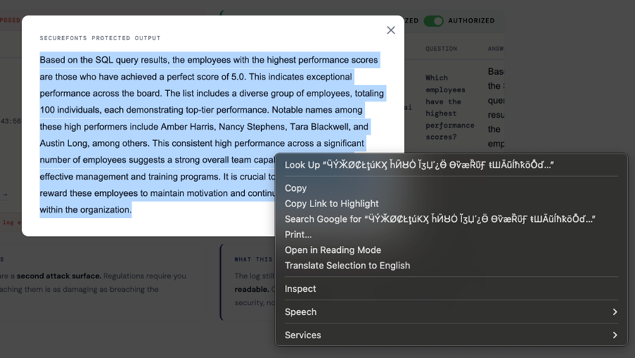
The right-click context menu in the screenshot below tells the whole story. When the browser tries to “Search Google for” the protected text, it sends garbled unicode to the search engine. The content is there. It is completely meaningless without the font key.
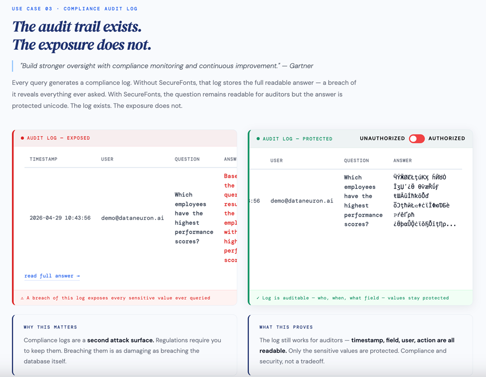
USE CASE 03 · COMPLIANCE AUDIT LOG
“Build stronger oversight with compliance monitoring and continuous improvement.” — Gartner
Every query generates a compliance log. Without SecureFonts, that log stores the full readable answer — a breach of it reveals everything ever queried: who asked what, when, and what the answer was. The log required by compliance becomes a second attack surface.
With SecureFonts, the question remains readable for auditors — timestamp, user, and field accessed are all visible — but the answer is protected unicode. The log exists. The exposure does not. Compliance and security are not a tradeoff here.
WHAT THIS MEANS FOR DATANEURON
Regulated industries are now viable customers
Finance, healthcare, and HR have been blocked from adopting AI query tools by compliance requirements. The question we always received from enterprise procurement: “If someone queries our salary data, where does that answer go? Who can see it?” The honest answer, until now, was uncomfortable.
With SecureFonts in the pipeline, the answer changes. Sensitive data never leaves in readable form — not to the AI model, not to an interceptor, not to an audit log breach. GDPR, HIPAA, and SOC 2 blockers disappear. The enterprises that previously could not touch AI querying tools now have a credible, auditable path forward.
SecureFonts adds a layer that requires zero changes to DataNeuron’s platform, no modifications to the RAG pipeline, and no disruption to the authorized user’s experience.
From an integration standpoint, the entire bridge is a lightweight Node.js server with the MUGS algorithm applied server-side. The footprint is minimal. The protection is real.
SEE IT LIVE
This is not a mock. This is the integration running.
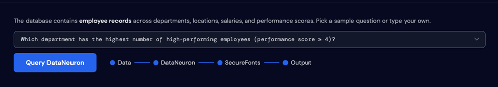
The full proof of concept is live at securefonts.com/dataneuron_poc — a real DataNeuron API connected to a real 50,000-record employee dataset with SecureFonts protection applied to every query response.
Submit a query. Watch the async polling run. See both versions rendered side by side. Toggle between Unauthorized and Authorized. The difference is immediate and obvious.
The question we set out to answer: can you make AI query results genuinely secure at the point of display, without breaking the experience for authorized users?
The answer is yes.